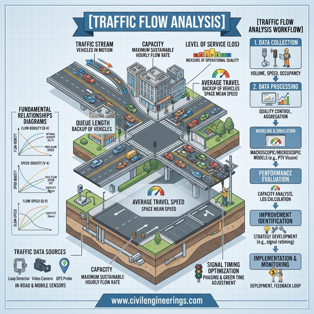
Traffic congestion rarely happens by accident. It usually develops when traffic demand approaches or exceeds the capacity of a road, intersection, or highway facility. Understanding how vehicles move, interact, slow down, queue, and recover is therefore essential for effective transportation planning. This is where Traffic Flow Analysis becomes an important part of highway and transportation engineering.

Traffic Flow Analysis studies the relationships among traffic volume, speed, density, headway, spacing, and roadway capacity. Engineers use these relationships to evaluate existing roads, predict operational problems, design new facilities, improve intersections, and select suitable traffic management measures.

For civil engineering students, it provides the foundation for understanding highway capacity and traffic operations. For highway engineers, consultants, contractors, and government agencies, it supports practical decisions involving road widening, intersection improvements, lane management, signal timing, and transportation planning.

This guide explains the fundamental traffic-flow parameters, important formulas, traffic-flow models, data collection techniques, capacity concepts, practical applications, and engineering best practices. It also discusses how principles associated with IRC, AASHTO, and ICE guidance can support professional traffic studies.

What Is Traffic Flow Analysis?

Traffic Flow Analysis is the systematic study of how vehicles and road users move through a transportation facility under particular roadway, traffic, and environmental conditions.

The analysis examines three fundamental traffic characteristics:

• Traffic volume or flow
• Traffic speed
• Traffic density

These variables are closely related. A change in one can significantly influence the others.

For example, a highway may carry a large number of vehicles while traffic remains relatively smooth when demand is below capacity. As demand increases, vehicle spacing decreases and drivers become more affected by the behavior of vehicles ahead. Eventually, congestion can develop, reducing average speed and increasing travel time.

Traffic-flow analysis helps engineers answer practical questions such as:

• How many vehicles use a road during the peak hour?
• What is the average travel speed?
• How densely packed are vehicles?
• What is the roadway’s practical capacity?
• When will congestion occur?
• How long will queues become?
• Would an additional lane improve operations?
• How will a proposed development affect traffic?
• Is an intersection operating satisfactorily?

Why Traffic Flow Analysis Is Important

Traffic-flow analysis forms a bridge between traffic data and engineering decisions. Without reliable analysis, road improvements may address symptoms rather than the actual operational problem.

Highway Planning and Design

Traffic forecasts help engineers determine the number of lanes, roadway classification, intersection requirements, median arrangements, and access-control strategies.

A road designed without adequate consideration of future traffic demand can become congested much earlier than expected.

Capacity Assessment

Engineers compare traffic demand with available roadway capacity. This allows them to determine whether an existing facility can accommodate present and projected traffic.

The basic relationship is:

Degree of Saturation = Traffic Demand / Capacity

When demand approaches capacity, traffic conditions become increasingly sensitive to disturbances such as lane changes, slow vehicles, merging, incidents, and poor weather.

Traffic Congestion Management

Traffic-flow analysis can identify the source and location of congestion. Possible improvements may include:

• Additional lanes
• Intersection redesign
• Signal optimization
• Access management
• Turning restrictions
• Ramp metering
• Public transport priority
• Intelligent transportation systems
• Work-zone traffic management

Road Safety

Traffic conditions influence crash risk. Large speed differences, frequent lane changes, unstable queues, and poorly managed merging areas can create safety concerns.

Traffic-flow studies help engineers identify locations where operational improvements may also produce safety benefits.

Fundamental Parameters of Traffic Flow

Three variables form the foundation of traffic-flow theory: flow, speed, and density.

Traffic Flow or Volume

Traffic flow represents the number of vehicles passing a reference point during a specified period.

The general equation is:

q = N / T

Where:

• q = traffic flow rate
• N = number of vehicles counted
• T = observation period

For example, if 900 vehicles pass a location in 15 minutes:

q = 900 / 0.25 = 3,600 vehicles/hour

The hourly flow rate is therefore 3,600 vehicles per hour.

Traffic counts may be classified by vehicle type, direction, lane, or movement.

Traffic Speed

Speed describes how quickly vehicles travel along a roadway.

Common measures include:

• Spot speed
• Time mean speed
• Space mean speed
• Running speed
• Travel speed
• Design speed

The distinction between time mean speed and space mean speed is particularly important in traffic engineering.

Time mean speed represents the arithmetic average of vehicle speeds observed at a particular point.

Space mean speed represents the average speed of vehicles over a road section and is generally more appropriate for travel-time analysis.

Traffic Density

Density represents the number of vehicles occupying a unit length of roadway at a given time.

The standard relationship is:

k = N / L

Where:

• k = density
• N = number of vehicles
• L = length of roadway section

Density is usually expressed as vehicles per kilometer per lane.

For example, if 90 vehicles occupy a 3-km road section:

k = 90 / 3 = 30 vehicles/km

Density provides a useful indication of how closely vehicles are packed.

Fundamental Relationship Between Flow, Speed, and Density

One of the most important relationships in traffic engineering is:

q = k × v

Where:

• q = flow
• k = density
• v = average speed

This relationship allows engineers to understand how traffic conditions change as demand increases.

For example, if:

• Density = 35 vehicles/km
• Average speed = 60 km/h

Then:

q = 35 × 60 = 2,100 vehicles/hour

The equation looks simple, but its engineering interpretation is important. Increasing density does not always increase flow. Once the roadway approaches its critical operating condition, additional density can cause speed to fall significantly and eventually reduce total flow.

Traffic Headway and Spacing

Traffic headway and spacing describe how vehicles are separated from one another.

Time Headway

Time headway is the time interval between two successive vehicles passing a reference point.

If 60 vehicles pass a point in one minute, the approximate average headway is:

h = 60 / q

When flow is expressed in vehicles per hour:

h = 3,600 / q

For a flow of 1,800 vehicles/hour:

h = 3,600 / 1,800 = 2 seconds

Average headway therefore equals approximately two seconds.

Vehicle Spacing

Spacing represents the distance between successive vehicles along a roadway.

It is influenced by:

• Vehicle speed
• Driver behavior
• Reaction time
• Road geometry
• Traffic density
• Weather
• Vehicle characteristics

Headway and spacing are especially useful when studying following behavior, platoons, queue formation, and roadway capacity.

Traffic Flow Characteristics

Traffic does not always behave in the same way. Engineers commonly examine three broad traffic-flow conditions.

Uninterrupted Flow

Uninterrupted flow occurs when traffic movement is not regularly interrupted by external controls.

Examples include:

• Freeways
• Expressways
• Rural highways
• Long highway sections without signals

Although incidents and congestion can still interrupt traffic, the facility itself does not routinely stop vehicles.

Interrupted Flow

Interrupted flow occurs when traffic is affected by control devices or external interruptions.

Typical examples include:

• Signalized intersections
• Stop-controlled intersections
• Pedestrian crossings
• Railway crossings
• Roundabouts

Queueing and delay become major components of the analysis.

Mixed Traffic Flow

Mixed traffic is particularly important in many developing transportation systems. Cars may share the same roadway with motorcycles, buses, trucks, rickshaws, bicycles, pedestrians, and other road users.

Different vehicle dimensions, speeds, acceleration capabilities, and lane-use behaviors can make conventional homogeneous traffic assumptions less reliable.

Engineers may use passenger car equivalents or similar adjustment concepts to represent mixed traffic effects.

Traffic Flow Models

Traffic-flow models help engineers predict how traffic responds to roadway and demand conditions.

Greenshields Model

The Greenshields model is one of the classical traffic-flow models. It assumes a linear relationship between speed and density.

A simplified expression is:

v = vf (1 − k/kj)

Where:

• v = average speed
• vf = free-flow speed
• k = density
• kj = jam density

The corresponding flow relationship can be expressed as:

q = k × vf (1 − k/kj)

The model is useful for teaching fundamental traffic-flow concepts, although real-world traffic often behaves more irregularly than the assumptions of a simple linear model.

Fundamental Diagram

A traffic fundamental diagram typically relates:

• Flow and density
• Speed and density
• Flow and speed

The flow-density curve generally rises as traffic demand increases, reaches a maximum flow at capacity, and then falls when congestion becomes severe.

A simplified representation is:

Traffic Flow
    |
    |                 Capacity
    |                    /\
    |                   /  \
    |                  /    \
    |                 /      \
    |________________/________\________ Density
                   Critical     Jam
                   Density     Density

The point of maximum flow represents the approximate capacity condition under the assumptions of the selected model.

Traffic Capacity and Level of Service

Roadway capacity is the maximum sustainable flow rate that a facility can reasonably accommodate under specified roadway, traffic, and control conditions.

Capacity depends on factors such as:

• Number of lanes
• Lane width
• Road alignment
• Grades
• Heavy vehicles
• Driver population
• Access points
• Traffic control
• Weather
• Roadside development
• Directional distribution

Capacity should not be treated as one universal number. It is a function of the facility and operating conditions.

Level of Service

Level of Service, commonly abbreviated as LOS, provides a framework for describing operating quality.

Depending on the facility and methodology, LOS evaluations may consider:

• Speed
• Density
• Delay
• Volume-to-capacity ratio
• Queue length
• Freedom to maneuver
• Travel-time reliability

The traditional LOS framework generally uses categories from A through F, with A representing relatively favorable operating conditions and F representing highly congested or breakdown conditions.

Engineers should use the appropriate current methodology rather than applying generic LOS thresholds without considering facility type and local conditions.

Traffic Data Collection Methods

Good traffic analysis begins with good data. Poor counts can lead to poor design decisions.

Manual Traffic Counts

Observers record vehicles using:

• Tally sheets
• Mobile applications
• Video recordings
• Classification forms

Manual counting works well for short-duration studies, intersection turning movements, and locations with unusual vehicle types.

Automatic Traffic Counters

Automatic systems can continuously record traffic using technologies such as:

• Inductive loops
• Pneumatic tubes
• Radar
• Video detection
• Infrared sensors
• Bluetooth or other tracking technologies

These systems are particularly useful when engineers need longer observation periods.

Origin-Destination Surveys

Origin-destination surveys identify where trips begin and end.

They can help determine:

• Travel patterns
• Through traffic
• Local traffic
• Diversion opportunities
• Freight movement
• Future corridor requirements

Turning Movement Counts

At intersections, engineers normally record movements such as:

• Through
• Left turn
• Right turn
• U-turn where applicable

The information supports intersection capacity analysis, signal design, lane assignment, and geometric improvements.

Peak Hour and Design Hour Traffic

Traffic changes throughout the day. Morning and evening commuter periods often produce significant demand.

A traffic study should identify appropriate peak periods rather than simply relying on an arbitrary one-hour count.

The Peak Hour Factor (PHF) is commonly used to describe traffic variation within the peak hour.

A common equation is:

PHF = Peak Hour Volume / (4 × Peak 15-Minute Volume)

Suppose the peak-hour volume is 2,000 vehicles and the highest 15-minute volume is 560 vehicles:

PHF = 2,000 / (4 × 560)

PHF = 0.893

A lower PHF indicates more concentrated traffic within the peak hour, while a value closer to 1.00 indicates a more uniform flow.

Passenger Car Equivalent in Traffic Analysis

Heavy vehicles can affect traffic flow differently from passenger cars because of their size, acceleration characteristics, braking behavior, and effects on other drivers.

The Passenger Car Equivalent (PCE) concept represents the effect of a particular vehicle type in terms of an equivalent number of passenger cars under specified conditions.

A simple mixed-traffic conversion may be represented as:

Equivalent Flow = Σ (Ni × PCEi)

Where:

• Ni = number of vehicles of type i
• PCEi = passenger car equivalent for vehicle type i

The actual PCE values should come from the applicable design methodology and local traffic conditions. Engineers should avoid blindly applying values from another country or roadway environment.

Traffic Queue Analysis

Queues develop when arriving traffic temporarily exceeds the service rate of a facility.

Common locations include:

• Signalized intersections
• Toll plazas
• Work zones
• Highway bottlenecks
• Ramp terminals
• Railway crossings

Queue analysis can examine:

• Average queue
• Maximum queue
• Queue duration
• Arrival rate
• Departure rate
• Delay
• Queue clearance time

Consider a signalized intersection where vehicles arrive at a rate greater than the rate at which the signal allows them to depart. The queue grows during the red phase and may dissipate during green. If the arrival demand remains too high, the queue may continue growing from one cycle to the next.

This distinction is important because a short temporary queue is very different from a recurring oversaturated queue.

Traffic Flow at Intersections

Intersections often represent the controlling point of an urban road network.

Traffic-flow analysis at intersections considers:

• Approach volume
• Turning movements
• Lane configuration
• Signal timing
• Saturation flow
• Pedestrian activity
• Heavy vehicles
• Right-of-way control
• Queue storage
• Approach speed

For signalized intersections, engineers examine green time, cycle length, phase sequence, lost time, saturation flow, and arrival patterns.

For unsignalized intersections, gap acceptance and conflicting traffic streams become especially important.

Practical Intersection Example

Suppose an intersection approach experiences high right-turn demand while through traffic remains moderate.

Simply widening the entire approach may not be the most efficient solution.

A better analysis might determine whether:

• A dedicated turning lane is required.
• Signal phasing should be modified.
• Storage length is adequate.
• Pedestrian crossing timing creates excessive delay.
• Access points upstream are contributing to conflicts.

This illustrates why traffic-flow analysis should precede geometric improvements.

Traffic Flow Analysis for Highway Projects

During highway development, traffic analysis can influence almost every stage of the project.

Planning Stage

At the planning stage, engineers assess:

• Existing traffic
• Historical growth
• Future demand
• Origin-destination patterns
• Freight movement
• Network connectivity
• Alternative corridors

Design Stage

Traffic information supports decisions about:

• Lane requirements
• Median design
• Interchanges
• Intersections
• Auxiliary lanes
• Service roads
• Access management
• Pavement design traffic

Construction Stage

Traffic analysis becomes important when existing traffic must pass through an active construction zone.

Engineers may evaluate:

• Lane closures
• Detours
• Temporary traffic signals
• Work-zone capacity
• Queue formation
• Traffic-control plans
• Emergency access

Operation and Maintenance Stage

After construction, traffic monitoring helps determine whether the facility is performing as expected.

Observed traffic can be compared with:

• Design assumptions
• Forecast demand
• Capacity
• Travel-time targets
• Safety objectives

Traffic Flow Analysis and Traffic Simulation

For complex networks, analytical equations alone may not adequately represent traffic behavior.

Microscopic and macroscopic simulation models can provide additional insight.

Simulation

Microscopic models represent individual vehicles and their interactions.

They can examine:

• Car-following
• Lane changing
• Merging
• Signal response
• Queue development
• Individual vehicle trajectories

Macroscopic Simulation

Macroscopic models treat traffic as a stream rather than tracking every vehicle individually.

They are useful for:

• Corridor-level analysis
• Network planning
• Demand assessment
• Large-scale congestion studies

Simulation should not replace engineering judgment. A model is only as useful as its input data, assumptions, calibration, and validation.

Role of IRC, AASHTO, and ICE Guidance

Professional traffic studies should follow the standards and guidance applicable to the project jurisdiction.

In India and many South Asian projects, engineers may refer to relevant Indian Roads Congress (IRC) publications for traffic studies, highway capacity, geometric design, traffic control, and related transportation engineering practices.

In the United States and projects influenced by American practice, AASHTO publications provide widely used guidance covering highway design, transportation planning, geometric considerations, and related engineering principles.

The Institution of Civil Engineers (ICE) provides professional guidance and knowledge resources relevant to infrastructure, transportation, engineering management, and sustainable infrastructure practice.

These organizations should not be treated as interchangeable design codes. Engineers must identify the contractual requirements, governing national standards, road authority requirements, and project-specific specifications before selecting analytical procedures.

Common Mistakes in Traffic Flow Analysis

Even technically sophisticated projects can suffer from basic data and interpretation problems.

Using Short or Unrepresentative Counts

A single day’s count may not represent typical traffic.

Engineers should consider:

• Weekday variation
• Weekend traffic
• Seasonal variation
• Holidays
• Special events
• Weather
• School schedules
• Construction activity

Ignoring Heavy Vehicles

Truck and bus percentages can materially influence traffic operations, especially on grades and constrained highway sections.

Applying Inappropriate Capacity Values

Capacity varies with facility type and conditions. A capacity figure from a freeway should not automatically be applied to a two-lane rural highway or urban arterial.

Treating Forecasts as Certainties

Traffic forecasts contain uncertainty. Scenario analysis can provide a more realistic understanding of possible future demand.

Poor Model Calibration

Simulation models should be calibrated against observed conditions such as:

• Flow
• Speed
• Travel time
• Queue length
• Saturation behavior

An attractive simulation output is not proof that the model is correct.

Best Practices for Traffic Flow Analysis

A reliable study should follow a disciplined process.

1. Define the objective.
Determine whether the study addresses capacity, congestion, safety, development impact, intersection operation, or future planning.

2. Identify the study area.
Include upstream and downstream locations that can influence the problem.

3. Collect representative data.
Use appropriate traffic counts, speed surveys, classification counts, turning movements, and travel-time observations.

4. Check data quality.
Look for missing records, unusual traffic conditions, equipment errors, and inconsistent observations.

5. Establish existing conditions.
Document roadway geometry, traffic control, traffic demand, speed, queues, and operational constraints.

6. Select the appropriate analytical method.
Use analytical equations, capacity procedures, intersection methods, or simulation according to the complexity of the problem.

7. Analyze future conditions.
Include traffic growth, development traffic, network changes, and planned infrastructure.

8. Test alternatives.
Compare improvements rather than assuming that road widening is always the answer.

9. Validate results.
Where possible, compare calculated or simulated conditions with field observations.

10. Document assumptions.
A professional report should clearly state data sources, analysis periods, adjustment factors, methodology, limitations, and recommendations.

Practical Recommendations for Civil Engineering Students

Students should focus on understanding relationships rather than memorizing formulas.

Start with:

• Flow
• Speed
• Density
• Headway
• Spacing
• Capacity
• Level of Service
• PHF
• PCE

Then practice solving numerical problems using realistic traffic-count data.

A useful student exercise is to record traffic for 15-minute intervals, calculate hourly flow, determine PHF, estimate average speed, and investigate how flow changes with density.

Learning spreadsheet analysis is also valuable. Modern highway engineers routinely work with large traffic datasets.

Practical Recommendations for Highway Engineers and Consultants

Engineers should treat field observations as an essential part of the analysis.

Before recommending additional lanes, investigate whether congestion is actually caused by:

• Bottleneck geometry
• Poor signal coordination
• Turning movements
• Access conflicts
• Merging
• Lane imbalance
• Heavy vehicles
• Construction activity

Use sensitivity analysis when future demand is uncertain.

For major projects, document assumptions carefully so that another engineer can reproduce the analysis.

Practical Recommendations for Contractors

Contractors may not perform long-term transportation planning, but traffic-flow principles remain important during construction.

Before implementing a traffic-control plan, consider:

• Existing peak traffic
• Lane closure capacity
• Queue storage
• Worker safety
• Emergency vehicle access
• Temporary signs
• Nighttime operations
• Detour routes
• Public access

Temporary traffic management should be reviewed as construction stages change. A traffic plan that worked during earthwork may not work during pavement construction when work zones, equipment movements, and lane availability change.

Frequently Asked Questions About Traffic Flow Analysis

What is Traffic Flow Analysis?

Traffic Flow Analysis is the study of vehicle movement and interaction using parameters such as traffic volume, speed, density, headway, capacity, and delay.

What are the three main parameters of traffic flow?

The three fundamental parameters are flow, speed, and density. Their basic relationship is expressed as q = k × v.

Why is traffic density important?

Density indicates how closely vehicles occupy a roadway. It helps engineers understand congestion, vehicle interactions, capacity conditions, and breakdown of traffic flow.

What is the difference between traffic flow and traffic volume?

The terms are often used interchangeably, but traffic flow commonly emphasizes a rate, such as vehicles per hour, while traffic volume may refer to the total number of vehicles counted during a particular period.

What is Peak Hour Factor?

Peak Hour Factor measures the variation of traffic within the peak hour. It is commonly calculated using peak-hour volume and the highest 15-minute volume.

What is roadway capacity?

Roadway capacity is the maximum sustainable traffic flow that a facility can reasonably accommodate under specified roadway, traffic, control, and environmental conditions.

What causes traffic flow to break down?

Breakdown can result when demand approaches or exceeds capacity. Incidents, merging, lane changes, poor weather, work zones, bottlenecks, and sudden driver behavior can also trigger unstable flow.

Is traffic simulation necessary for every project?

No. Smaller projects may be adequately evaluated using field observations and established analytical procedures. Simulation becomes more useful when traffic interactions or network complexity make conventional analysis insufficient.

How does traffic-flow analysis improve road design?

It helps determine lane requirements, intersection configurations, signal strategies, access arrangements, capacity needs, queue storage, and operational improvements.

Which standards should engineers use for traffic-flow studies?

Engineers should use the standards specified by the relevant road authority and project jurisdiction. IRC, AASHTO, and ICE resources can provide valuable professional guidance, but the applicable contractual and national requirements should always govern the final methodology.

Conclusion

Traffic Flow Analysis is one of the fundamental tools used to understand, design, operate, and improve transportation facilities. It connects field traffic observations with engineering decisions by examining flow, speed, density, headway, capacity, delay, queues, and traffic interactions.

A reliable analysis begins with representative data and continues through appropriate calculations, capacity evaluation, modeling, validation, and engineering judgment. The objective should not simply be to calculate how many vehicles use a road. Engineers need to understand why traffic behaves the way it does and what practical intervention can improve the transportation system.

For students, mastering the fundamental relationships provides a strong foundation in highway engineering. For professionals, accurate traffic analysis supports better decisions about road widening, intersections, work zones, traffic management, and future infrastructure.

As transportation networks become more complex, combining traditional traffic engineering with data collection, intelligent transportation systems, simulation, and evidence-based planning will become increasingly important. A well-executed traffic-flow study ultimately helps create roads that are safer, more efficient, more reliable, and better prepared for future demand.