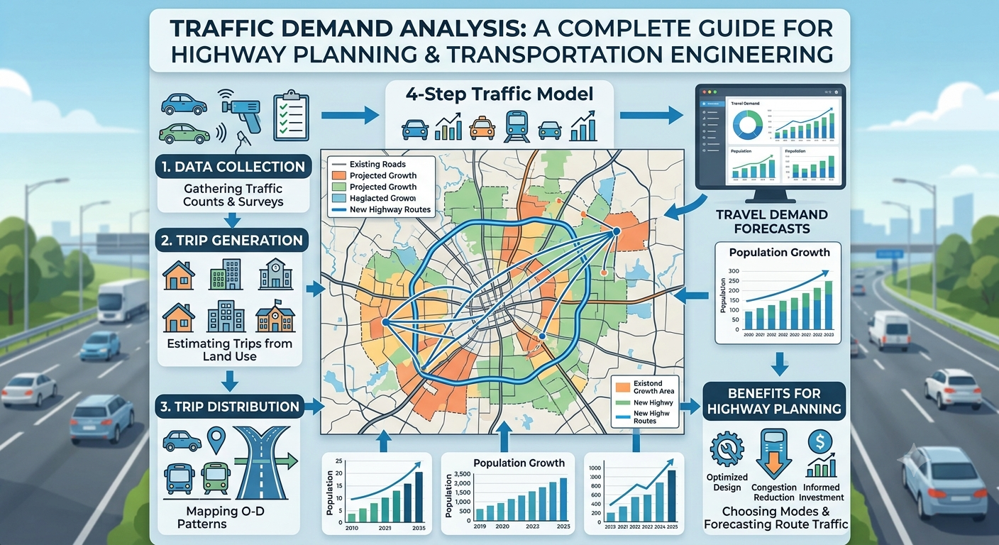
Modern roads are expected to serve more than today’s traffic. A highway, urban arterial, bypass, interchange, or new development must also accommodate the travel demand that may develop years after construction. That is why engineers cannot rely only on existing traffic counts when deciding roadway capacity, number of lanes, intersection improvements, or future transportation investment.

Traffic Demand Analysis provides a systematic way to understand how many trips people and goods generate, where those trips go, which modes they use, and how they distribute themselves across a transportation network. It combines traffic surveys, land-use information, demographic data, economic indicators, travel behavior, and transportation modeling to develop a realistic picture of present and future demand.

For highway engineers and transportation planners, the analysis becomes particularly important during route selection, feasibility studies, pavement and geometric design, interchange planning, congestion assessment, and economic evaluation. FHWA describes travel demand forecasting as a process focused on future travel demand and notes that future AADT forecasts can rely on extensive traffic and travel-demand modeling inputs. (Federal Highway Administration)

This guide explains the complete process, major methods, formulas, data requirements, forecasting techniques, practical examples, model calibration, common mistakes, and professional best practices.

What Is Traffic Demand Analysis?

Traffic Demand Analysis is the engineering process of estimating, understanding, and forecasting the amount and pattern of travel generated by people, businesses, freight activities, and land uses within a defined study area.

In simple terms, it answers four fundamental questions:

1. How many trips will be made?
2. Where will those trips start and end?
3. Which transportation mode will travelers choose?
4. Which routes or facilities will carry those trips?

These questions form the foundation of transportation planning.

A demand analysis may examine an existing road corridor or a completely new transportation facility. The study can range from a small intersection or development access road to a metropolitan highway network.

Unlike a simple traffic count, demand analysis looks beyond observed vehicles. It attempts to explain why traffic exists and how traffic may change when population, employment, land use, income, vehicle ownership, travel costs, road capacity, or transportation policies change.

FHWA identifies travel demand models as tools that can represent trip generation, destination choice, mode choice, time-of-day choice, and route choice based on land-use, socioeconomic, and transportation-network characteristics. (Federal Highway Administration)

Why Traffic Demand Analysis Is Important

Traffic demand analysis influences many decisions throughout a road or highway project’s life cycle.

Highway Capacity Planning

Engineers need future traffic volumes to determine whether a proposed road requires two lanes, four lanes, six lanes, or additional capacity in the future.

A road designed only for current traffic may become congested prematurely. Conversely, excessive capacity can increase construction costs and result in inefficient use of public funds.

Geometric Design

Traffic demand affects decisions regarding:

• Lane requirements
• Carriageway width
• Intersection configuration
• Turning lanes
• Median design
• Interchange requirements
• Auxiliary lanes
• Access management
• Pedestrian and bicycle facilities
• Design-hour traffic

Traffic forecasts therefore connect transportation planning with geometric highway design.

Pavement Design

Forecast traffic is also essential for pavement engineering. Heavy commercial vehicles contribute substantially to pavement deterioration, so engineers need information about:

• Average daily traffic
• Commercial vehicle percentage
• Axle configurations
• Directional distribution
• Lane distribution
• Traffic growth
• Design period

These inputs can ultimately influence cumulative design traffic and pavement thickness.

Economic Evaluation

A transportation project may generate benefits through:

• Travel-time savings
• Vehicle operating cost reductions
• Improved reliability
• Accident reduction
• Reduced congestion
• Freight efficiency
• Improved accessibility

Traffic demand forecasts provide the foundation for estimating many of these benefits.

Land-Use and Development Planning

Large residential communities, shopping centers, industrial zones, universities, airports, hospitals, and business districts can generate substantial traffic.

A development traffic study can estimate the additional trips and determine whether surrounding roads and intersections can accommodate them.

Traffic Demand Analysis Data Requirements

Reliable analysis starts with reliable data. Poor input data can produce technically sophisticated but misleading forecasts.

Traffic Volume Data

Typical traffic count data include:

• Hourly traffic volume
• Daily traffic volume
• Peak-hour volume
• Directional traffic
• Vehicle classification
• Turning movements
• Seasonal variations

Important indicators include AADT, peak-hour volume, directional split, and percentage of heavy vehicles.

For example:$$AADT = \frac{\text{Annual Traffic Volume}}{365}$$

If only short-duration counts are available, appropriate adjustment factors may be required to estimate representative annual conditions.

Origin-Destination Data

Origin-destination, or O-D, information identifies where trips begin and end.

Common sources include:

• Household travel surveys
• Roadside interviews
• Automatic number-plate recognition
• Bluetooth/Wi-Fi observations
• GPS data
• Mobile-device datasets
• Freight surveys
• Existing transportation models

An O-D matrix can then represent travel between traffic analysis zones.

Socioeconomic Data

Travel demand is strongly influenced by socioeconomic conditions.

Useful variables include:

• Population
• Households
• Employment
• Household income
• Vehicle ownership
• Students
• Workers
• Commercial activity
• Industrial activity
• Land-use type

FHWA forecasting work similarly recognizes demographic and economic factors as important explanatory variables for vehicle travel. (Federal Highway Administration)

Transportation Network Data

The network model should represent relevant characteristics such as:

• Road classification
• Number of lanes
• Road capacity
• Speed
• Intersection controls
• Travel time
• Turn restrictions
• Toll costs
• Road hierarchy
• Public transport services
• Major bottlenecks

Route choice can be influenced by distance, travel time, speed, tolls, and other forms of impedance. (Federal Highway Administration)

Traffic Demand Analysis Process

A professional study generally follows a structured sequence rather than jumping directly from traffic counts to a future volume.

Define the Study Area

First establish the geographical limits of the analysis.

The study area should be large enough to capture important traffic generators, competing routes, major intersections, development areas, and network changes.

For a highway project, the study may include:

• Project corridor
• Parallel routes
• Connecting arterials
• Major intersections
• Interchanges
• Residential areas
• Commercial centers
• Industrial zones

A narrow study boundary can overlook diverted or redistributed traffic.

Establish Existing Conditions

The next step is to understand the existing transportation system.

Engineers typically document:

• Existing AADT
• Peak-hour traffic
• Speed
• Travel time
• Intersection delays
• Level of service
• Road geometry
• Traffic controls
• Crash history
• Public transport
• Pedestrian and bicycle activity

Existing conditions form the baseline against which future scenarios are compared.

Identify Traffic Generators

Traffic generators are land uses or activities that produce or attract trips.

Examples include:

• Housing developments
• Shopping malls
• Offices
• Factories
• Schools
• Universities
• Hospitals
• Airports
• Railway stations
• Logistics centers

The scale and type of development influence both the number and characteristics of trips.

Estimate Trip Generation

Trip generation determines the number of trips produced and attracted by each zone or land-use category.

A simple relationship may be represented as:$$T = R \times X$$

Where:

• $T$ = estimated trips
• $R$ = trip-generation rate
• $X$ = relevant land-use variable

For a residential project, $X$ might represent households. For an office development, it could represent employees or floor area.

In professional studies, trip rates should be selected from appropriate local studies, accepted manuals, agency guidance, or calibrated models rather than copied blindly from another location.

Perform Trip Distribution

Trip distribution determines where generated trips travel.

The output is generally represented as an origin-destination matrix.

One common conceptual approach is the gravity model:$$T_{ij}=K \frac{P_i A_j f(c_{ij})}{\sum_j A_j f(c_{ij})}$$

Where:

• $T_{ij}$ = trips from origin $i$ to destination $j$
• $P_i$ = trips produced at origin $i$
• $A_j$ = trips attracted to destination $j$
• $c_{ij}$ = travel impedance
• $f(c_{ij})$ = impedance function
• $K$ = balancing factor

The impedance function may account for travel time, distance, generalized cost, or other resistance to travel.

Trip distribution is one of the more challenging components of travel modeling because small errors in destination patterns can affect downstream traffic assignments. FHWA notes that destination choice/trip distribution has historically been a major source of error in travel modeling systems. (Federal Highway Administration)

Determine Mode Choice

Travelers may select different transportation modes.

Typical modes include:

• Private car
• Motorcycle
• Bus
• Rail
• Walking
• Bicycle
• Ride-sharing
• Other shared mobility

Mode choice depends on factors such as:

• Travel time
• Cost
• Income
• Vehicle ownership
• Transit availability
• Parking cost
• Convenience
• Accessibility
• Reliability

Ignoring mode shift can overestimate future automobile demand in areas where public transportation or active transportation is expanding.

Perform Traffic Assignment

Traffic assignment places estimated trips onto the transportation network.

The assignment process attempts to determine which routes travelers are likely to use.

Inputs can include:

• O-D matrix
• Road network
• Travel time
• Capacity
• Toll
• Intersection delay
• Route impedance

The output may include:

• Link traffic volumes
• Route flows
• Volume-to-capacity ratios
• Travel times
• Congestion
• Network performance

FHWA distinguishes travel demand models from HCM-based tools: demand models focus on changes in travel demand, while HCM-type tools are generally used to analyze facility or bottleneck performance rather than predict demand changes themselves. (Federal Highway Administration)

The Four-Step Travel Demand Model

One of the best-known frameworks for Traffic Demand Analysis is the traditional four-step model.

Trip Generation

The model estimates trips produced and attracted by each zone.

Typical inputs include:

• Population
• Households
• Employment
• Income
• Vehicle ownership
• Land use

Trip Distribution

Generated trips are connected between origins and destinations.

The result is commonly an O-D matrix.

Mode Choice

Trips are divided among available transportation modes.

For example, a future scenario might show:

• 70% private vehicles
• 15% public transport
• 10% walking
• 5% cycling and other modes

Actual proportions must come from appropriate local data or a validated model.

Traffic Assignment

The final step loads trips onto the network.

The resulting traffic volumes can then support highway capacity analysis, intersection analysis, pavement traffic estimation, and transportation investment decisions.

FHWA’s more recent modeling guidance notes that activity-based models are increasingly used alongside or instead of traditional trip-based four-step models because they can represent individual and household activity patterns in greater detail. (Federal Highway Administration)

Traffic Growth and Future Demand Forecasting

Future traffic forecasting is central to highway planning.

A simple growth-rate method can be written as:$$V_f = V_0(1+g)^n$$

Where:

• $V_f$ = future traffic
• $V_0$ = base-year traffic
• $g$ = annual growth rate
• $n$ = number of years

Example

Suppose an existing highway carries:$$V_0 = 25,000\ vehicles/day$$

Assume an annual growth rate of:$$g = 4\%$$

and a design period of:$$n = 15\ years$$

Then:$$V_f = 25,000(1.04)^{15}$$

The resulting demand is approximately 45,000 vehicles/day.

This simple calculation is useful for preliminary assessment, but professional forecasting should not automatically assume a constant growth rate. Major changes in land use, fuel prices, economic activity, public transportation, road capacity, and travel behavior can alter the growth pattern.

Compound Annual Growth Rate

Historical traffic trends can also be examined using:$$CAGR = \left(\frac{V_f}{V_0}\right)^{1/n}-1$$

Historical growth should be reviewed carefully. A sudden increase may reflect a new development rather than a permanent regional trend.

Peak-Hour Traffic Analysis

Roadway capacity is not determined by daily traffic alone.

Two roads can have the same AADT but substantially different peak-hour characteristics.

Important parameters include:

• Peak Hour Volume
• Directional Distribution
• Peak Hour Factor
• Heavy Vehicle Percentage
• Lane Distribution

Peak Hour Factor can be calculated as:$$PHF = \frac{V}{4V_{15}}$$

Where:

• $V$ = hourly volume
• $V_{15}$ = highest 15-minute volume within that hour

A lower PHF indicates a more concentrated peak flow.

For highway design, engineers may also use a design-hour volume concept:$$DHV = K \times AADT$$

where $K$ represents the relationship between the design-hour volume and AADT.

The appropriate values depend on the project, location, traffic characteristics, and governing design guidance.

Traffic Demand Analysis for New Roads

A new road has no historical traffic count at the facility itself, so engineers must estimate demand indirectly.

The analysis may consider:

Existing Parallel Routes

Traffic on nearby roads can indicate potential demand.

New Development

Planned housing, commercial, industrial, or institutional projects can create additional trips.

Route Diversion

A new road may attract traffic from existing routes because it offers:

• Shorter travel time
• Better pavement
• Greater capacity
• Improved safety
• Reduced congestion
• Lower toll
• Better connectivity

Induced and Redistributed Demand

Major capacity improvements can change travel behavior. Some travelers may shift routes, destinations, departure times, modes, or even make trips they previously avoided.

Therefore, simply adding the forecasted background growth to a new road may not accurately represent future demand.

Traffic Demand Analysis for Existing Roads

Existing corridors benefit from observed traffic data, but historical data still require careful interpretation.

Engineers should check:

• Count dates
• Seasonal conditions
• Weather
• Road construction
• Special events
• Holidays
• Temporary restrictions
• Economic changes
• Recent developments

Short-term counts should not automatically be treated as representative annual traffic.

FHWA specifically identifies historical and existing AADT as important inputs for travel demand model development, calibration, and validation. (Federal Highway Administration)

Model Calibration and Validation

A traffic model is not automatically reliable because it produces attractive maps and tables.

Calibration adjusts model parameters so that modeled behavior reasonably represents observed conditions.

Validation then tests the model against data that were not simply used to create it.

Useful comparison measures include:

• Observed versus modeled traffic volume
• Screenline flows
• Turning movements
• Travel times
• Route patterns
• V/C ratios
• Transit ridership
• O-D patterns

GEH Statistic

A commonly used traffic-volume comparison measure is the GEH statistic:$$GEH=\sqrt{\frac{2(M-C)^2}{M+C}}$$

Where:

• $M$ = modeled volume
• $C$ = observed count

The GEH statistic is useful for comparing modeled and observed traffic volumes during model checking. FHWA documentation also identifies GEH as a volume-accuracy measure for comparing predicted and field traffic volumes. (Highways)

Model calibration should never become an exercise in forcing every modeled number to match one traffic count. The objective is to achieve a credible representation of travel behavior and network conditions.

Traffic Demand Analysis Tools and Software

Different tools are appropriate for different questions.

Spreadsheet and Statistical Tools

Useful for:

• Growth calculations
• Traffic trend analysis
• Trip-generation calculations
• Sensitivity testing
• Preliminary forecasting

GIS

Geographic Information Systems help visualize:

• Traffic zones
• Road networks
• Land use
• Population
• Employment
• Traffic generators
• Development patterns

Travel Demand Models

These are appropriate for large-scale forecasting and network planning.

They can evaluate:

• Future traffic
• Route changes
• Network alternatives
• Mode shifts
• Land-use scenarios
• Long-term transportation plans

Microsimulation

Microsimulation is more appropriate when detailed operational behavior is required at intersections, corridors, or localized networks.

FHWA emphasizes that different analysis tools serve different geographic scales and purposes; travel demand models are particularly suited to system-level demand forecasting, while simulation tools can provide more detailed facility and bottleneck analysis. (Federal Highway Administration)

Traffic Demand Analysis and Capacity Analysis: What Is the Difference?

These two concepts are related but not identical.

Traffic demand describes how much travel users want to make.

Capacity describes how much traffic a transportation facility can reasonably serve under defined conditions.

For example:

• Forecast demand = 4,000 vehicles/hour
• Available capacity = 3,000 vehicles/hour

The demand exceeds capacity.

This does not mean the roadway will physically carry 4,000 vehicles/hour under all circumstances. Congestion, queuing, rerouting, time shifting, and other behavioral responses may occur.

That distinction is important when interpreting traffic forecasts.

Common Mistakes in Traffic Demand Analysis

Using One Traffic Count as the Forecast

A single count cannot explain an entire traffic system.

Applying an Unverified Growth Rate

A historical 5% growth rate does not guarantee another 5% annual increase for the next 20 years.

Ignoring Heavy Vehicles

Truck traffic can significantly influence highway performance and pavement requirements.

Ignoring Competing Routes

A new highway can redistribute traffic from existing roads.

Ignoring Land-Use Changes

Future development can dramatically alter travel patterns.

Treating Model Output as Reality

A model is an analytical representation. Engineers must apply professional judgment and compare results with observed conditions.

Mixing Demand and Operations Models

A travel demand model and a detailed intersection simulation do not serve exactly the same purpose. FHWA recommends selecting analysis tools according to the project stage and analytical question. (Federal Highway Administration)

IRC, AASHTO, and ICE Guidance

Traffic Demand Analysis should always follow the standards and guidance applicable to the project’s jurisdiction.

IRC

In India and many South Asian engineering environments, relevant Indian Roads Congress (IRC) publications can provide guidance related to traffic surveys, highway planning, traffic studies, geometric design, capacity, and transportation planning.

AASHTO

In the United States and projects influenced by U.S. practice, AASHTO guidance is commonly used alongside FHWA resources for highway planning and design. AASHTO publications should be applied according to the specific project type and governing agency requirements.

ICE

The Institution of Civil Engineers (ICE) provides professional guidance and engineering knowledge relevant to transportation infrastructure, planning, risk, sustainability, and project delivery.

These organizations should not be treated as interchangeable. Engineers should identify the governing authority, applicable edition, local standards, project requirements, and contractual specifications before selecting design parameters.

Practical Recommendations for Students, Engineers, and Contractors

For Civil Engineering Students

Build a strong foundation in:

• Traffic volume studies
• AADT
• Peak-hour analysis
• Trip generation
• Trip distribution
• Mode choice
• Traffic assignment
• Highway capacity
• Transportation planning
• GIS
• Basic statistics

Do not focus only on software. Understand what each model is actually calculating.

For Highway and Traffic Engineers

Always establish a clear forecasting methodology.

Document:

• Base year
• Forecast years
• Traffic counts
• Growth assumptions
• Land-use assumptions
• Network assumptions
• Mode-share assumptions
• Model calibration
• Validation results
• Sensitivity scenarios

A transparent model is easier to review, update, and defend.

For Contractors

Traffic demand forecasts can influence construction staging and temporary traffic management.

Contractors should understand expected:

• Construction traffic
• Detour volumes
• Work-zone traffic
• Heavy vehicle movements
• Access requirements
• Temporary capacity restrictions

Poorly planned construction traffic can create operational problems even when the permanent highway design is adequate.

For Consultants and Government Engineers

Do not rely on a single forecast.

Develop sensitivity cases such as:

• Low-growth scenario
• Base-growth scenario
• High-growth scenario
• Major development scenario
• Public-transport improvement scenario
• Alternative network scenario

Scenario testing provides decision-makers with a better understanding of uncertainty.

Future Trends in Traffic Demand Analysis

Traffic forecasting is becoming more data-driven.

Modern transportation studies increasingly incorporate:

• GPS probe data
• Mobile-device data
• Connected vehicle information
• Artificial intelligence
• Machine learning
• Real-time traffic feeds
• Automated traffic counts
• Activity-based models
• Dynamic traffic assignment
• Multimodal modeling
• Big-data analytics

Modern modeling can also operate at multiple levels of resolution. FHWA’s multiresolution guidance discusses the relationship between travel demand models, static traffic assignment, dynamic traffic assignment, microsimulation, and other modeling approaches. (Federal Highway Administration)

The future is not simply about collecting more data. The real objective is to combine better data with sound transportation theory, transparent assumptions, and appropriate engineering judgment.

FAQs About Traffic Demand Analysis

What is Traffic Demand Analysis?

Traffic Demand Analysis is the process of estimating current and future travel demand and understanding how trips are generated, distributed, assigned, and divided among transportation modes.

Why is Traffic Demand Analysis important in highway design?

It helps engineers estimate future traffic, determine roadway capacity, evaluate alternatives, plan intersections and interchanges, and support pavement and economic analyses.

What are the four steps of travel demand modeling?

The traditional four steps are trip generation, trip distribution, mode choice, and traffic assignment.

What is the difference between traffic demand and traffic capacity?

Demand represents the amount of travel users seek to make, while capacity represents the amount of traffic a facility can serve under specified conditions.

What data are required for traffic forecasting?

Typical data include traffic counts, AADT, O-D information, population, employment, land use, vehicle ownership, travel time, road-network characteristics, and socioeconomic information.

How is future traffic volume calculated?

A basic approach uses compound growth:$$V_f=V_0(1+g)^n$$

However, major projects should consider land-use changes, network changes, socioeconomic trends, and alternative scenarios.

What is traffic assignment?

Traffic assignment allocates estimated origin-destination trips to available transportation routes based on network characteristics such as travel time, distance, capacity, and cost.

Can GIS be used in Traffic Demand Analysis?

Yes. GIS is highly useful for mapping traffic zones, land use, population, employment, road networks, traffic generators, and forecast results.

What is model calibration?

Calibration adjusts model parameters so the model reproduces observed travel behavior and traffic conditions within acceptable limits.

Is Traffic Demand Analysis required for every road project?

Not necessarily at the same level of detail. A minor local road may need a relatively simple traffic assessment, while a major highway, interchange, bypass, or large development may require comprehensive travel demand modeling.

Conclusion

Traffic Demand Analysis is one of the most important foundations of modern transportation planning and highway engineering. A roadway should not be designed simply around the number of vehicles observed today. Engineers must understand where trips originate, where they are going, why travelers choose particular modes and routes, and how these patterns may change in the future.

A sound analysis combines traffic counts, origin-destination information, socioeconomic data, land-use forecasts, transportation networks, travel behavior, and appropriate modeling techniques. The traditional four-step framework remains valuable, while activity-based modeling, dynamic assignment, probe data, GIS, and advanced analytics are expanding the capabilities available to transportation professionals.

The most important lesson is simple: a traffic model is only as reliable as its data, assumptions, calibration, validation, and engineering judgment. Students should learn the principles before software. Engineers should document assumptions. Consultants should test uncertainty. Government agencies should demand transparent forecasts. Contractors should understand how projected demand affects construction staging and traffic management.

When these practices are combined, Traffic Demand Analysis becomes much more than a forecasting exercise. It becomes a decision-making framework for developing safer, more efficient, economical, and future-ready transportation infrastructure. (Federal Highway Administration)